Welcome to DYNAMAX!#
Dynamax is a library for probabilistic state space models (SSMs) written in JAX. It has code for inference (state estimation) and learning (parameter estimation) in a variety of SSMs, including:
Hidden Markov Models (HMMs)
Linear Gaussian State Space Models (aka Linear Dynamical Systems)
Nonlinear Gaussian State Space Models
Generalized Gaussian State Space Models (with non-Gaussian emission models)
The library consists of a set of core, functionally pure, low-level inference algorithms, as well as a set of model classes which provide a more user-friendly, object-oriented interface. It is compatible with other libraries in the JAX ecosystem, such as optax (used for estimating parameters using stochastic gradient descent), and Blackjax (used for computing the parameter posterior using Hamiltonian Monte Carlo (HMC) or sequential Monte Carlo (SMC)).
Installation and Testing#
To install the latest releast of dynamax from PyPi:
pip install dynamax                 # Install dynamax and core dependencies, or
pip install dynamax[notebooks]      # Install with demo notebook dependencies
To install the latest development branch:
pip install git+https://github.com/probml/dynamax.git
Finally, if you’re a developer, you can install dynamax along with the test and documentation dependencies with:
git clone git@github.com:probml/dynamax.git
cd dynamax
pip install -e '.[dev]'
To run the tests:
pytest dynamax                         # Run all tests
pytest dynamax/hmm/inference_test.py   # Run a specific test
pytest -k lgssm                        # Run tests with lgssm in the name
What are state space models?#
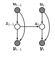
A state space model or SSM is a partially observed Markov model, in which the hidden state, \(z_t\), evolves over time according to a Markov process, possibly conditional on external inputs / controls / covariates, \(u_t\), and generates an observation, \(y_t\). This is illustrated in the graphical model below.
The corresponding joint distribution has the following form (in dynamax, we restrict attention to discrete time systems):
Here \(p(z_t \mid z_{t-1}, u_t)\) is called the transition or dynamics model, and \(p(y_t \mid z_{t}, u_t)\) is called the observation or emission model. (In both cases, the inputs \(u_t\) are optional; furthermore, the observation model may have auto-regressive dependencies, in which case we write \(p(y_t \mid z_{t}, u_t, y_{1:t-1})\).)
We assume that we see the observations \(y_{1:T}\), and want to infer the hidden states, either using online filtering (i.e., computing \(p(z_t \mid y_{1:t})\)) or offline smoothing (i.e., computing \(p(z_t \mid y_{1:T})\)). We may also be interested in predicting future states, \(p(z_{t+h} \mid y_{1:t})\), or future observations, \(p(y_{t+h} \mid y_{1:t})\), where h is the forecast horizon. (Note that by using a hidden state to represent the past observations, the model can have “infinite” memory, unlike a standard auto-regressive model.) All of these computations can be done efficiently using Dynamax. Moreover, you can use Dynamax to estimate the parameters of the transition and emission models, as we discuss below.
More information can be found in these books:
“Machine Learning: Advanced Topics”, K. Murphy, MIT Press 2023. Available at https://probml.github.io/pml-book/book2.html.
“Bayesian Filtering and Smoothing, Second Edition”, S. Särkkä and L. Svensson, Cambridge University Press, 2023. Available at http://users.aalto.fi/~ssarkka/pub/bfs_book_2023_online.pdf
Quickstart#
Dynamax includes classes for many kinds of SSM. You can use these models to simulate data, and you can fit the models using standard learning algorithms like expectation-maximization (EM) and stochastic gradient descent (SGD). Below we illustrate the high level (object-oriented) API for the case of an HMM with Gaussian emissions. (See this notebook for a runnable version of this code.)
import jax.numpy as jnp
import jax.random as jr
import matplotlib.pyplot as plt
from dynamax.hidden_markov_model import GaussianHMM

key1, key2, key3 = jr.split(jr.PRNGKey(0), 3)
num_states = 3
emission_dim = 2
num_timesteps = 1000

# Make a Gaussian HMM and sample data from it
hmm = GaussianHMM(num_states, emission_dim)
true_params, _ = hmm.initialize(key1)
true_states, emissions = hmm.sample(true_params, key2, num_timesteps)

# Make a new Gaussian HMM and fit it with EM
params, props = hmm.initialize(key3, method="kmeans", emissions=emissions)
params, lls = hmm.fit_em(params, props, emissions, num_iters=20)

# Plot the marginal log probs across EM iterations
plt.plot(lls)
plt.xlabel("EM iterations")
plt.ylabel("marginal log prob.")

# Use fitted model for posterior inference
post = hmm.smoother(params, emissions)
print(post.smoothed_probs.shape) # (1000, 3)
JAX allows you to easily vectorize these operations with vmap. For example, you can sample and then fit to a batch of emissions as shown below.
from functools import partial
from jax import vmap

num_seq = 200
batch_true_states, batch_emissions = \
   vmap(partial(hmm.sample, true_params, num_timesteps=num_timesteps))(
      jr.split(key2, num_seq))
print(batch_true_states.shape, batch_emissions.shape) # (200,1000) and (200,1000,2)

# Make a new Gaussian HMM and fit it with EM
params, props = hmm.initialize(key3, method="kmeans", emissions=batch_emissions)
params, lls = hmm.fit_em(params, props, batch_emissions, num_iters=20)
You can also call the low-level inference code (e.g. hmm_smoother()) directly,
without first having to construct the HMM object.
Tutorials#
The tutorials below will introduce you to state space models in Dynamax. If you’re new to these models, we recommend you start at the top and work your way through!
HMMs
Linear Gaussian SSMs
Nonlinear Gaussian SSMs