Tracking a 1d pendulum using Extended / Unscented Kalman filter/ smoother

This notebook demonstrates a simple pendulum tracking example. The example is taken from p45 of Bayesian Filtering and Smoothing (S. Särkkä, 2013). This code is based on the sarkka-jax repo.

The physics of the problem is shown below, where \(\alpha\) is the angle relative to vertical, and \(w(t)\) is a white noise process added to the angular velocity (a random acceleration term).

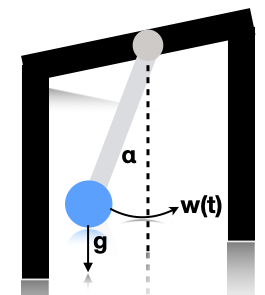
This gives rise to the following differential equation:

\[\begin{align*} \frac{d^2 \alpha}{d t^2} = -g \sin(\alpha) + w(t) \end{align*}\]

We can write this as a nonlinear SSM by defining the state to be \(z_1(t) = \alpha(t)\) and \(z_2(t) = d\alpha(t)/dt\). Thus

\[\begin{align*} \frac{d z}{dt} = \begin{pmatrix} z_2 \\ -g \sin(z_1) \end{pmatrix} + \begin{pmatrix} 0 \\ 1 \end{pmatrix} w(t) \end{align*}\]

If we discretize this step size \(\Delta\), we get the following formulation:

\[\begin{align*} \begin{pmatrix} z_{1,t} \\ z_{2,t} \end{pmatrix} = \begin{pmatrix} z_{1,t-1} + z_{2,t-1} \Delta \\ z_{2,t-1} -g \sin(z_{1,t-1}) \Delta \end{pmatrix} +q_{t} \end{align*}\]

where \(q_t \sim N(0,Q)\), and

\[\begin{equation*} Q = q^c \begin{pmatrix} \frac{\Delta^3}{3} & \frac{\Delta^2}{2} \\ \frac{\Delta^2}{2} & \Delta \end{pmatrix} \end{equation*}\]

where \(q^c\) is the spectral density of the continuous-time noise process.

We assume the observation model is

\[\begin{align*} y_t &= h(z_t) + r_t \\ h(z_t) &= \sin(\alpha_t) = \sin(z_{t,1}) \\ r_t &\sim N(0,R) \end{align*}\]

Setup

%%capture
try:
    import dynamax
except ModuleNotFoundError:
    print('installing dynamax')
    %pip install -q dynamax[notebooks]
    import dynamax

%matplotlib inline
import matplotlib.pyplot as plt

import jax.numpy as jnp
import jax.random as jr
from jax import lax
from jaxtyping import Float, Array
from typing import Callable, NamedTuple

from dynamax.nonlinear_gaussian_ssm import ParamsNLGSSM, UKFHyperParams
from dynamax.nonlinear_gaussian_ssm import extended_kalman_smoother, unscented_kalman_smoother

# For pretty print of ndarrays
jnp.set_printoptions(formatter={"float_kind": "{:.2f}".format})

Sample data and plot it

# Some parameters
dt = 0.0125
g = 9.8
q_c = 1
r = 0.3

# Lightweight container for pendulum parameters
class PendulumParams(NamedTuple):
    initial_state: Float[Array, "state_dim"] = jnp.array([jnp.pi / 2, 0])
    dynamics_function: Callable = lambda x: jnp.array([x[0] + x[1] * dt, x[1] - g * jnp.sin(x[0]) * dt])
    dynamics_covariance: Float[Array, "state_dim state_dim"] = jnp.array([[q_c * dt**3 / 3, q_c * dt**2 / 2], [q_c * dt**2 / 2, q_c * dt]])
    emission_function: Callable = lambda x: jnp.array([jnp.sin(x[0])])
    emission_covariance: Float[Array, "emission_dim"] = jnp.eye(1) * (r**2)

# Pendulum simulation (Särkkä Example 3.7)
def simulate_pendulum(params=PendulumParams(), key=0, num_steps=400):
    if isinstance(key, int):
        key = jr.PRNGKey(key)
    # Unpack parameters
    M, N = params.initial_state.shape[0], params.emission_covariance.shape[0]
    f, h = params.dynamics_function, params.emission_function
    Q, R = params.dynamics_covariance, params.emission_covariance

    def _step(carry, rng):
        state = carry
        rng1, rng2 = jr.split(rng, 2)

        next_state = f(state) + jr.multivariate_normal(rng1, jnp.zeros(M), Q)
        obs = h(next_state) + jr.multivariate_normal(rng2, jnp.zeros(N), R)
        return next_state, (next_state, obs)

    rngs = jr.split(key, num_steps)
    _, (states, observations) = lax.scan(_step, params.initial_state, rngs)
    return states, observations


states, obs = simulate_pendulum()

def plot_pendulum(time_grid, x_tr, x_obs, x_est=None, est_type=""):
    plt.figure()
    plt.plot(time_grid, x_tr, color="darkgray", linewidth=4, label="True Angle")
    plt.plot(time_grid, x_obs, "ok", fillstyle="none", ms=1.5, label="Measurements")
    if x_est is not None:
        plt.plot(time_grid, x_est, color="k", linewidth=1.5, label=f"{est_type} Estimate")
    plt.xlabel("Time $t$")
    plt.ylabel("Pendulum angle $x_{1,k}$")
    plt.xlim(0, 5)
    plt.ylim(-3, 5)
    plt.xticks(jnp.arange(0.5, 4.6, 0.5))
    plt.yticks(jnp.arange(-3, 5.1, 1))
    plt.gca().set_aspect(0.5)
    plt.legend(loc=1, borderpad=0.5, handlelength=4, fancybox=False, edgecolor="k")
    plt.show()

# Create time grid for plotting
time_grid = jnp.arange(0.0, 5.0, step=dt)

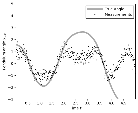
# Plot the generated data
plot_pendulum(time_grid, states[:, 0], obs)

# Compute RMSE
def compute_rmse(y, y_est):
    return jnp.sqrt(jnp.sum((y - y_est) ** 2) / len(y))


# Compute RMSE of estimate and print comparison with
# standard deviation of measurement noise
def compute_and_print_rmse_comparison(y, y_est, R, est_type=""):
    rmse_est = compute_rmse(y, y_est)
    print(f'{f"The RMSE of the {est_type} estimate is":<40}: {rmse_est:.2f}')
    print(f'{"The std of measurement noise is":<40}: {jnp.sqrt(R):.2f}')

Extended Kalman Filter / smoother

pendulum_params = PendulumParams()

# Define parameters for EKF
ekf_params = ParamsNLGSSM(
    initial_mean=pendulum_params.initial_state,
    initial_covariance=jnp.eye(states.shape[-1]) * 0.1,
    dynamics_function=pendulum_params.dynamics_function,
    dynamics_covariance=pendulum_params.dynamics_covariance,
    emission_function=pendulum_params.emission_function,
    emission_covariance=pendulum_params.emission_covariance,
)

ekf_posterior = extended_kalman_smoother(ekf_params, obs)

m_ekf = ekf_posterior.filtered_means[:, 0]
plot_pendulum(time_grid, states[:, 0], obs, x_est=m_ekf, est_type="EKF")
compute_and_print_rmse_comparison(states[:, 0], m_ekf, r, "EKF")

The RMSE of the EKF estimate is         : 0.14
The std of measurement noise is         : 0.55

m_ekf = ekf_posterior.smoothed_means[:, 0]
plot_pendulum(time_grid, states[:, 0], obs, x_est=m_ekf, est_type="EKS")
compute_and_print_rmse_comparison(states[:, 0], m_ekf, r, "EKS")

The RMSE of the EKS estimate is         : 0.09
The std of measurement noise is         : 0.55

Unscented Kalman Filter / smoother

pendulum_params = PendulumParams()

ukf_params = ParamsNLGSSM(
    initial_mean=pendulum_params.initial_state,
    initial_covariance=jnp.eye(states.shape[-1]) * 0.1,
    dynamics_function=pendulum_params.dynamics_function,
    dynamics_covariance=pendulum_params.dynamics_covariance,
    emission_function=pendulum_params.emission_function,
    emission_covariance=pendulum_params.emission_covariance,
)

ukf_hyperparams = UKFHyperParams() # default gives same results as EKF


ukf_posterior = unscented_kalman_smoother(ukf_params, obs, ukf_hyperparams)

m_ukf = ukf_posterior.filtered_means[:, 0]
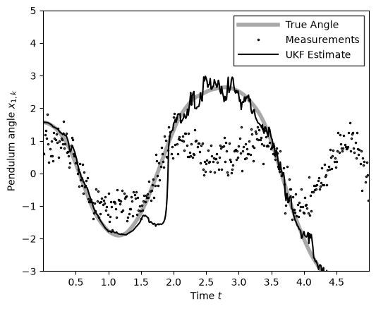
plot_pendulum(time_grid, states[:, 0], obs, x_est=m_ukf, est_type="UKF")
compute_and_print_rmse_comparison(states[:, 0], m_ukf, r, "UKF")

The RMSE of the UKF estimate is         : 0.14
The std of measurement noise is         : 0.55

m_uks = ukf_posterior.smoothed_means[:, 0]
plot_pendulum(time_grid, states[:, 0], obs, x_est=m_uks, est_type="UKS")
compute_and_print_rmse_comparison(states[:, 0], m_uks, r, "UKS")

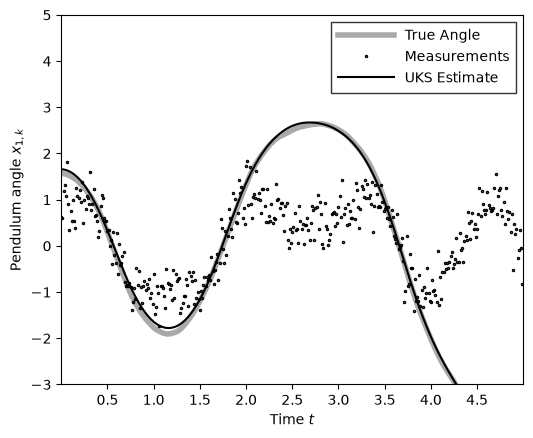
The RMSE of the UKS estimate is         : 0.09
The std of measurement noise is         : 0.55

# Let's see how sensitive UKF is to hyper-params

ukf_hyperparams = UKFHyperParams(alpha=3, beta=3, kappa=3)

ukf_posterior = unscented_kalman_smoother(ukf_params, obs, ukf_hyperparams)

m_ukf = ukf_posterior.filtered_means[:, 0]
plot_pendulum(time_grid, states[:, 0], obs, x_est=m_ukf, est_type="UKF")
compute_and_print_rmse_comparison(states[:, 0], m_ukf, r, "UKF")

The RMSE of the UKF estimate is         : 1.07
The std of measurement noise is         : 0.55