Casino HMM: Learning (parameter estimation)#
This notebook continues the “occasionally dishonest casino” example from the preceding notebook. There, we assumed we knew the parameters of the model: the probability of switching between fair and loaded dice and the probabilities of the different outcomes (1,…,6) for each die.
Here, our goal is learn these parameters from data. We will sample data from the model as before, but now we will estimate the parameters using either stochastic gradient descent (SGD) or expectation-maximization (EM).
The figure below shows the graphical model, complete with the parameter nodes.
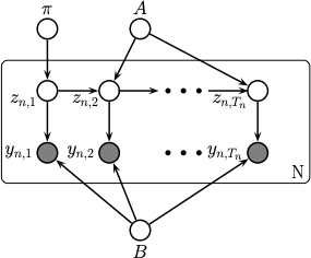
In Dynamax, the CategoricalHMM assumes conjugate, Dirichlet prior distributions on the model parameters. Let \(K\) denote the number of discrete states (\(K=2\) in the casino example, either fair or loaded), and let \(C\) the number of categories the emissions can assume (\(C=6\) in the casino example, the number of faces of each die). The priors are:
Thus, the full prior distribution is,
The hyperparameters can be specified in the CategoricalHMM constructor.
The learning objective is to find parameters that maximize the marginal probability,
This is called the maximum a posteriori (MAP) estimate. Dynamax supports two algorithms for MAP estimation: expectation-maximization (EM) and stochastic gradient descent (SGD), which are described below.
Setup#
from functools import partial

import jax.numpy as jnp
import jax.random as jr
import matplotlib.pyplot as plt
import optax
from jax import vmap

from dynamax.hidden_markov_model import CategoricalHMM
Sample data from true model#
First we construct an HMM and sample data from it, just as in the preceding notebook.
num_states = 2      # two types of dice (fair and loaded)
num_emissions = 1   # only one die is rolled at a time
num_classes = 6     # each die has six faces

initial_probs = jnp.array([0.5, 0.5])
transition_matrix = jnp.array([[0.95, 0.05],
                               [0.10, 0.90]])
emission_probs = jnp.array([[1/6,  1/6,  1/6,  1/6,  1/6,  1/6],    # fair die
                            [1/10, 1/10, 1/10, 1/10, 1/10, 5/10]])  # loaded die


# Construct the HMM
hmm = CategoricalHMM(num_states, num_emissions, num_classes)

# Initialize the parameters struct with known values
params, _ = hmm.initialize(initial_probs=initial_probs,
                           transition_matrix=transition_matrix,
                           emission_probs=emission_probs.reshape(num_states, num_emissions, num_classes))
num_batches = 5
num_timesteps = 5000
hmm = CategoricalHMM(num_states, num_emissions, num_classes)

batch_states, batch_emissions = \
    vmap(partial(hmm.sample, params, num_timesteps=num_timesteps))(
        jr.split(jr.PRNGKey(42), num_batches))

print(f"batch_states.shape:    {batch_states.shape}")
print(f"batch_emissions.shape: {batch_emissions.shape}")
batch_states.shape:    (5, 5000)
batch_emissions.shape: (5, 5000, 1)
We’ll write a simple function to print the parameters in a more digestible format.
def print_params(params):
    jnp.set_printoptions(formatter={'float': lambda x: "{0:0.3f}".format(x)})
    print("initial probs:")
    print(params.initial.probs)
    print("transition matrix:")
    print(params.transitions.transition_matrix)
    print("emission probs:")
    print(params.emissions.probs[:, 0, :]) # since num_emissions = 1

print_params(params)
initial probs:
[0.500 0.500]
transition matrix:
[[0.950 0.050]
 [0.100 0.900]]
emission probs:
[[0.167 0.167 0.167 0.167 0.167 0.167]
 [0.100 0.100 0.100 0.100 0.100 0.500]]
Learning with Gradient Descent#
Perhaps the simplest learning algorithm is to directly maximize the marginal probability with gradient ascent. Since optimization algorithms are typically formulated as minimization algorithms, we will instead use gradient descent to solve the equivalent problem of minimizing the negative log marginal probability, \(-\log p(y_{1:T}, \theta)\). On each iteration, we compute the objective, take its gradient, and update our parameters by taking a step in the direction of steepest descent.
Note
Automatic Differentiation Even though JAX code looks just like regular numpy code, it supports automatic differentiation, making gradient descent straightforward to implement.
Note
Initialization
The first step is to randomly initialize new parameters. You can do that by calling hmm.initialize(key),
where key is a JAX pseudorandom number generator (PRNG) key. When no other keyword arguments are supplied, this function will return parameters randomly sampled from the prior.
Note
Stick Transitions
Since we expect the states to persist for some time, we add a little stickiness to the prior distribution on transition probabilities via the transition_matrix_stickiness hyperparameter. This hyperparameter changes the prior to,
where \(\kappa \in \mathbb{R}_+\) is the stickiness paramter and \(e_k\) is the one-hot vector with a one in the \(k\)-th position.
Note
Handling Constraints Some of the HMM parameters have constraints. Dynamax uses bijectors to convert these parameters into unconstrained space for optimization. For example, the transition matrix must be a row-stochastic matrix, so we instead optimize an unconstrained, real-valued matrix and map it to a transition matrix via a `tfb.SoftmaxCentered bijector.
hmm = CategoricalHMM(num_states, num_emissions, num_classes,
                     transition_matrix_stickiness=10.0)

key = jr.PRNGKey(0)
init_params, props = hmm.initialize(key)

print("Randomly initialized parameters")
print_params(init_params)
Randomly initialized parameters
initial probs:
[0.635 0.365]
transition matrix:
[[0.920 0.080]
 [0.023 0.977]]
emission probs:
[[0.569 0.016 0.037 0.150 0.164 0.064]
 [0.127 0.141 0.070 0.306 0.058 0.298]]
Note
Notice that initialize returns two things, the parameters and their properties. Among other things, the properties allow you to specify which parameters should be learned. You can set the trainable flag to False if you want to fix certain parmeters.
Gradient descent is a special case of stochastic gradient descent#
Gradient descent is a special case of stochastic gradient descent (SGD) in which each iteration uses all the data to compute the descent direction for parameter updates. In contrast, SGD uses only a minibatch of data in each update. You can think of gradient descent as the special case where the minibatch is really the entire dataset. That’s why we sometimes call it full batch gradient descent. When you’re working with very large datasets (e.g. datasets with many sequences), however, minibatches can be very informative, and SGD can converge more quickly than full batch gradient descent.
Dynamax models have a fit_sgd function that runs SGD. If you want to run full batch gradient descent, all you have to do set batch_size=num_batches, as below.
fbgd_key = jr.PRNGKey(0)
fbgd_params, fbgd_losses = hmm.fit_sgd(init_params,
                                       props,
                                       batch_emissions,
                                       optimizer=optax.sgd(learning_rate=0.025, momentum=0.95),
                                       batch_size=num_batches,
                                       num_epochs=500,
                                       key=fbgd_key)
Stochastic Gradient Descent with Mini-Batches#
Now let’s run it with stochastic gradient descent using a batch size of two sequences per mini-batch.
sgd_key = jr.PRNGKey(0)
sgd_params, sgd_losses = hmm.fit_sgd(init_params,
                                     props,
                                     batch_emissions,
                                     optimizer=optax.sgd(learning_rate=0.025, momentum=0.95),
                                     batch_size=2,
                                     num_epochs=500,
                                     key=sgd_key)
Hyperparameter Tuning#
SGD and other optimizers like Adam have hyperparameters like the learning rate and momentum. For nonconvex optimization problems like these, the hyperparameters can make a big difference. We recommend sweeping over these parameters to find the most effective setting. Here, we show a simple grid search over the learning rate for Adam.
adam_key = jr.PRNGKey(0)
adam_learning_rates = [0.001, 0.01, 0.1, 0.25, 0.5]
adam_results = dict()
for lr in adam_learning_rates:
    print(f"Training with Adam, learning rate = {lr}")
    this_key, adam_key = jr.split(adam_key)
    these_params, these_losses = hmm.fit_sgd(init_params,
                                             props,
                                             batch_emissions,
                                             optimizer=optax.adam(learning_rate=lr),
                                             batch_size=2,
                                             num_epochs=500,
                                             key=this_key)

    adam_results[lr] = (these_params, these_losses)
Training with Adam, learning rate = 0.001
Training with Adam, learning rate = 0.01
Training with Adam, learning rate = 0.1
Training with Adam, learning rate = 0.25
Training with Adam, learning rate = 0.5
Learning with Expectation-Maximization (EM)#
The more traditional way to estimate the parameters of an HMM is by expectation-maximization (EM). EM alternates between two steps:
E-step: Inferring the posterior distribution of latent states \(z_{1:T}\) given the parameters \(\theta = (\pi, A, B)\). This step essentially runs the HMM forward-backward algorithm from the preceding notebook!
M-step: Updating the parameters to maximize the expected log probability. By iteratively performing these two steps, the algorithm converges to a local maximum of the marginal probability, \(p(y_{1:T}, \theta)\), and hence to a MAP estimate of the parameters.
EM often works very well for HMMs, especially when the models are “nice” (e.g. constructed with exponential family emission distributions) where the M-step can be computed in closed form. Dynamax has closed form M-steps for a variety of HMMs, including those with categorical observations and Gaussian observations with several different constraints on the covariance matrix. Please see our other demos for more examples!
key = jr.PRNGKey(0)
em_params, log_probs = hmm.fit_em(init_params,
                                  props,
                                  batch_emissions,
                                  num_iters=500)
Compare the learning algorithms#
Finally, let’s compare the learning curve of EM to those of gradient-based methods. For comparison, we plot the loss associated with the true parameters that generated the data.
Important
To compare the log probabilities returned by fit_em to the losses returned by fit_sgd, you need to negate the log probabilities and divide by the total number of emissions. This is because optimization library defaults typically assume the loss is scaled to be \(\mathcal{O}(1)\).
# Compute the "losses" from EM
em_losses = -log_probs / batch_emissions.size

# Compute the loss if you used the parameters that generated the data
true_loss = vmap(partial(hmm.marginal_log_prob, params))(batch_emissions).sum()
true_loss += hmm.log_prior(params)
true_loss = -true_loss / batch_emissions.size

# Plot the learning curves
plt.plot(fbgd_losses, label="full batch GD")
plt.plot(sgd_losses, label="SGD (m.b. size=2)")
for lr, (_, adam_losses) in adam_results.items():
    plt.plot(adam_losses, label=f"Adam (m.b. size=2, lr={lr})")
# plt.plot(adam_losses, label="Adam (mini-batch size = 2)")
plt.plot(em_losses, label="EM", color='k')
plt.axhline(true_loss, color='k', linestyle=':', label="True Params")
plt.legend()
plt.xlim(-10, 500)
plt.xlabel("epoch")
plt.ylabel("loss")
_ = plt.title("Learning Curve Comparison")
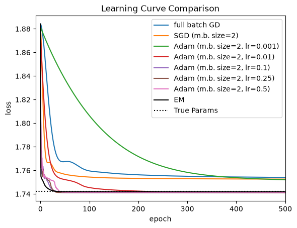
For this problem, EM and Adam with a well-tuned learning rate converge the fastest. SGD and full-batch gradient descent appear to get stuck in a local optimum. By contrast, EM and Adam match the loss under the true parameters, and indeed if we look at the parameters below, they nearly recover the true parameters up to label switching.
Note
Label Switching and Identifiability Label switching refers to the fact that the generated parameters assume state 1 corresponds to the loaded die, whereas the learned parameters assume this is state 0; since these solutions have the same likelihood, and since the prior is also symmetrical, there are two equally good posterior modes, and EM will just find one of them. When you compare inferred parameters or states between models, you may need to use our find_permutation function to find the best correspondence between discrete latent labels.
print("True Parameters:")
print_params(params)
print("")
print("EM Estimated Parameters:")
print_params(em_params)
print("")
print("Adam (lr=0.1) Estimated Parameters:")
print_params(adam_results[0.1][0])
True Parameters:
initial probs:
[0.500 0.500]
transition matrix:
[[0.950 0.050]
 [0.100 0.900]]
emission probs:
[[0.167 0.167 0.167 0.167 0.167 0.167]
 [0.100 0.100 0.100 0.100 0.100 0.500]]

EM Estimated Parameters:
initial probs:
[0.510 0.490]
transition matrix:
[[0.947 0.053]
 [0.082 0.918]]
emission probs:
[[0.167 0.171 0.169 0.172 0.166 0.156]
 [0.105 0.105 0.113 0.105 0.111 0.462]]

Adam (lr=0.1) Estimated Parameters:
initial probs:
[0.392 0.608]
transition matrix:
[[0.944 0.056]
 [0.086 0.914]]
emission probs:
[[0.164 0.170 0.172 0.175 0.166 0.153]
 [0.108 0.106 0.110 0.104 0.108 0.465]]
Conclusion#
This notebook showed how to learn the parameters of an HMM using gradient-based methods (with full batch or with mini-batches) and EM. For many HMMs, especially the exponential family HMMs with exact M-steps implemented in Dynamax, EM tends to converge very quickly.
This notebook glossed over some important details:
Both SGD and EM are prone to getting stuck in local optima. For example, if you change the key for the random initialization, you may find that the learned parameters are not as good. There are a few ways around that problem. One is to use a heuristic to initialize the parameters more intelligently. Another is to use many random initializations of the model and keep the one that achieves the best loss.
This notebook did not address the important question of how to determine the number of discrete states. We often use cross-validation for that purpose, as described next.
So far, we have focused on HMMs with discrete emissions from a categorical distribution. The next notebook will illustrate a Gaussian HMM for continuous data. We will also discuss some of the concerns above.