Tracking an object using the Kalman filter#
Consider an object moving in \(R^2\). We assume that we observe a noisy version of its location at each time step. We want to track the object and possibly forecast its future motion. We now show how to do this using a simple linear Gaussian SSM, combined with the Kalman filter algorithm.
Let the hidden state represent the position and velocity of the object, \(z_t =\begin{pmatrix} u_t & v_t & \dot{u}_t & \dot{v}_t \end{pmatrix}\). (We use \(u\) and \(v\) for the two coordinates, to avoid confusion with the state and observation variables.) The process evolves in continuous time, but if we discretize it with step size \(\Delta\), we can write the dynamics as the following linear system:
where \(q_t \in R^4\) is the process noise, which we assume is Gaussian, so \(q_t \sim N(0,Q)\).
Now suppose that at each discrete time point we observe the location (but not the velocity). We assume the observation is corrupted by Gaussian noise. Thus the observation model becomes
where \(r_t \sim N(0,R)\) is the observation noise. We see that the observation matrix \(H\) simply ``extracts’’ the relevant parts of the state vector.
Setup#
from jax import numpy as jnp
from jax import random as jr
from jax import vmap
from matplotlib import pyplot as plt

from dynamax.utils.plotting import plot_uncertainty_ellipses
from dynamax.linear_gaussian_ssm import LinearGaussianSSM
from dynamax.linear_gaussian_ssm import lgssm_smoother, lgssm_filter
Create the model#
state_dim = 4
emission_dim = 2
delta = 1.0

# Create object
lgssm = LinearGaussianSSM(state_dim, emission_dim)

# Manually chosen parameters
initial_mean = jnp.array([8.0, 10.0, 1.0, 0.0])
initial_covariance = jnp.eye(state_dim) * 0.1
dynamics_weights  = jnp.array([[1, 0, delta, 0],
                               [0, 1, 0, delta],
                               [0, 0, 1, 0],
                               [0, 0, 0, 1]])
dynamics_covariance = jnp.eye(state_dim) * 0.001
emission_weights = jnp.array([[1.0, 0, 0, 0],
                              [0, 1.0, 0, 0]])
emission_covariance = jnp.eye(emission_dim)

# Initialize model
params, _ = lgssm.initialize(jr.PRNGKey(0),
                             initial_mean=initial_mean,
                             initial_covariance=initial_covariance,
                             dynamics_weights=dynamics_weights,
                             dynamics_covariance=dynamics_covariance,
                             emission_weights=emission_weights,
                             emission_covariance=emission_covariance)
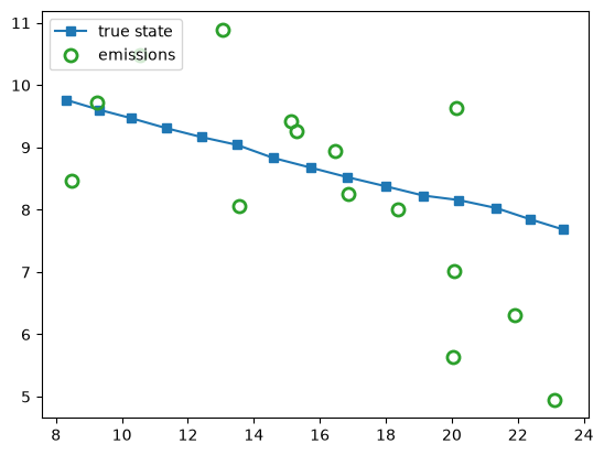
Sample some data from the model#
num_timesteps = 15
key = jr.PRNGKey(310)
x, y = lgssm.sample(params, key, num_timesteps)

# Plot Data
observation_marker_kwargs = {"marker": "o", "markerfacecolor": "none", "markeredgewidth": 2, "markersize": 8}
fig1, ax1 = plt.subplots()
ax1.plot(*x[:, :2].T, marker="s", color="C0", label="true state")
ax1.plot(*y.T, ls="", **observation_marker_kwargs, color="tab:green", label="emissions")
ax1.legend(loc="upper left")
<matplotlib.legend.Legend at 0x7f95902e04d0>
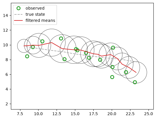
Perform online filtering#
lgssm_posterior = lgssm.filter(params, y)
print(lgssm_posterior.filtered_means.shape)
print(lgssm_posterior.filtered_covariances.shape)
print(lgssm_posterior.marginal_loglik)
(15, 4)
(15, 4, 4)
-51.273422
fig2, ax2 = plt.subplots()
ax2.plot(*y.T, ls="", **observation_marker_kwargs, color="tab:green", label="observed")
ax2.plot(*x[:, :2].T, ls="--", color="darkgrey", label="true state")
plot_lgssm_posterior(
    lgssm_posterior.filtered_means,
    lgssm_posterior.filtered_covariances,
    ax2,
    color="tab:red",
    label="filtered means",
    ellipse_kwargs={"edgecolor": "k", "linewidth": 0.5},
    legend_kwargs={"loc":"upper left"}
)
<Axes: >
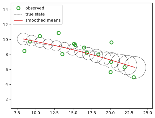
Perform offline smoothing#
lgssm_posterior = lgssm.smoother(params, y)
fig3, ax3 = plt.subplots()
ax3.plot(*y.T, ls="", **observation_marker_kwargs, color="tab:green", label="observed")
ax3.plot(*x[:, :2].T, ls="--", color="darkgrey", label="true state")
plot_lgssm_posterior(
    lgssm_posterior.smoothed_means,
    lgssm_posterior.smoothed_covariances,
    ax3,
    color="tab:red",
    label="smoothed means",
    ellipse_kwargs={"edgecolor": "k", "linewidth": 0.5},
    legend_kwargs={"loc":"upper left"}
)
<Axes: >
Low-level interface to the underlying inference algorithms#
We can also call the inference code directly, without having to make an LG-SSM object. We just pass the model parameters directly to the function.
filtered_posterior = lgssm_filter(params, y) # Kalman filter
smoothed_posterior = lgssm_smoother(params, y) # Kalman filter + smoother
assert jnp.allclose(lgssm_posterior.filtered_means, filtered_posterior.filtered_means)
assert jnp.allclose(lgssm_posterior.filtered_means, smoothed_posterior.filtered_means)
assert jnp.allclose(lgssm_posterior.smoothed_means, smoothed_posterior.smoothed_means)
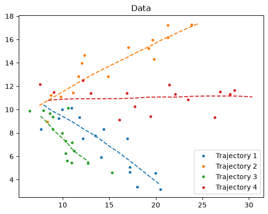
Tracking multiple objects in parallel#
# Generate 4 sample trajectories
num_timesteps = 15
num_samples = 4
key = jr.PRNGKey(310)
keys = jr.split(key, num_samples)
xs, ys = vmap(lambda key: lgssm.sample(params, key, num_timesteps))(keys)
# vmap the inference
lgssm_posteriors = vmap(lambda y: lgssm.smoother(params, y))(ys)
def plot_kf_parallel(xs, ys, lgssm_posteriors):
num_samples = len(xs)
dict_figures = {}
# Plot Data
fig, ax = plt.subplots()
for n in range(num_samples):
ax.plot(*xs[n, :, :2].T, ls="--", color=f"C{n}")
ax.plot(*ys[n, ...].T, ".", color=f"C{n}", label=f"Trajectory {n+1}")
ax.set_title("Data")
ax.legend()
dict_figures["missiles_latent"] = fig
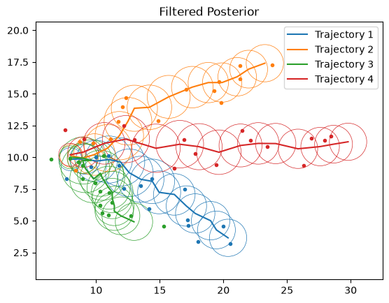
# Plot Filtering
fig, ax = plt.subplots()
for n in range(num_samples):
ax.plot(*ys[n, ...].T, ".")
filt_means = lgssm_posteriors.filtered_means[n, ...]
filt_covs = lgssm_posteriors.filtered_covariances[n, ...]
plot_lgssm_posterior(
filt_means,
filt_covs,
ax,
color=f"C{n}",
ellipse_kwargs={"edgecolor": f"C{n}", "linewidth": 0.5},
label=f"Trajectory {n+1}",
)
ax.legend(fontsize=10)
ax.set_title("Filtered Posterior")
dict_figures["missiles_filtered"] = fig
# Plot Smoothing
fig, ax = plt.subplots()
for n in range(num_samples):
ax.plot(*ys[n, ...].T, ".")
filt_means = lgssm_posteriors.smoothed_means[n, ...]
filt_covs = lgssm_posteriors.smoothed_covariances[n, ...]
plot_lgssm_posterior(
filt_means,
filt_covs,
ax,
color=f"C{n}",
ellipse_kwargs={"edgecolor": f"C{n}", "linewidth": 0.5},
label=f"Trajectory {n+1}",
)
ax.legend(fontsize=10)
ax.set_title("Smoothed Posterior")
dict_figures["missiles_smoothed"] = fig
return dict_figures
dict_figures = plot_kf_parallel(xs, ys, lgssm_posteriors)