Gaussian HMM: Cross-validation and Model Selection#
A Gaussian HMM has emissions of the form,
where the emission parameters \(\theta = \{(\mu_k, \Sigma_k)\}_{k=1}^K\) include the means and covariances for each of the \(K\) discrete states.
Dynamax implements a variety of Gaussian HMMs with different constraints on the parameters (e.g. diagonal, spherical, and tied covariances). It also includes prior distributions on the parameters. For example, it uses a conjugate normal-inverse Wishart (NIW) prior for the standard case.
This notebook shows how to:
Fit such models using expectation-maximization (EM)
Use cross-validation to choose the number of discrete states
Use the log probability of held-out data to choose among different models
Setup#
from functools import partial

import jax.numpy as jnp
import jax.random as jr
import matplotlib.pyplot as plt
from jax import vmap

from dynamax.hidden_markov_model import GaussianHMM
from dynamax.hidden_markov_model import DiagonalGaussianHMM
from dynamax.hidden_markov_model import SphericalGaussianHMM
from dynamax.hidden_markov_model import SharedCovarianceGaussianHMM
from dynamax.utils.plotting import CMAP, COLORS, white_to_color_cmap
Helper functions for plotting#
Generate sample data#
As in the preceding notebooks, we start by sampling data from the model. Here, we add a slight wrinkle: we will sample training and test data, where the latter is only used for model selection.
num_train_batches = 3
num_test_batches = 1
num_timesteps = 100

# Make an HMM and sample data and true underlying states
true_num_states = 5
emission_dim = 2
hmm = GaussianHMM(true_num_states, emission_dim)

# Specify parameters of the HMM
initial_probs = jnp.ones(true_num_states) / true_num_states
transition_matrix = 0.80 * jnp.eye(true_num_states) \
    + 0.15 * jnp.roll(jnp.eye(true_num_states), 1, axis=1) \
    + 0.05 / true_num_states
emission_means = jnp.column_stack([
    jnp.cos(jnp.linspace(0, 2 * jnp.pi, true_num_states + 1))[:-1],
    jnp.sin(jnp.linspace(0, 2 * jnp.pi, true_num_states + 1))[:-1],
    jnp.zeros((true_num_states, emission_dim - 2)),
    ])
emission_covs = jnp.tile(0.1**2 * jnp.eye(emission_dim), (true_num_states, 1, 1))

true_params, _ = hmm.initialize(initial_probs=initial_probs,
                                transition_matrix=transition_matrix,
                                emission_means=emission_means,
                                emission_covariances=emission_covs)

# Sample train, validation, and test data
train_key, val_key, test_key = jr.split(jr.PRNGKey(0), 3)
f = vmap(partial(hmm.sample, true_params, num_timesteps=num_timesteps))
train_true_states, train_emissions = f(jr.split(train_key, num_train_batches))
test_true_states,  test_emissions  = f(jr.split(test_key, num_test_batches))
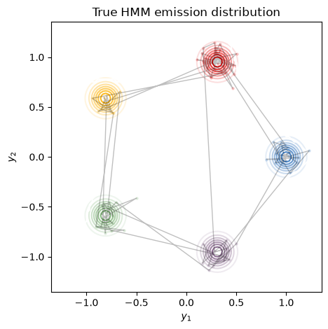
Here, we plot the emission distributions, \(p(x_t \mid z_t=k)\) for each \(k=1,\ldots, 5\). The gray dots indicate the observed points, \(x_t\), and the lines connect sequential observations. In this example, the transitions switch from blue to red to yellow and so on, since the transition matrix is constructed in a “feed-forward” fashion.
# Plot emissions and true_states in the emissions plane
plot_gaussian_hmm(hmm, true_params, train_emissions[0], train_true_states[0],
                  title="True HMM emission distribution")
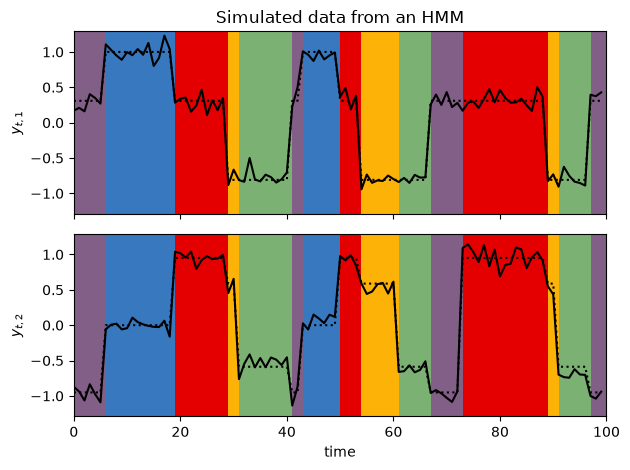
# Plot emissions vs. time with background colored by true state
plot_gaussian_hmm_data(hmm, true_params, train_emissions[0], train_true_states[0])
Write a helper function to perform leave-one-out cross-validation#
This function fits the data into folds where each fold consists of all but one of the training sequences. It fits the model to each fold in parallel, and then computes the log likelihood of the held-out sequence for each fold. The average held-out log likelihood is what we will use for determining the number of discrete states.
def cross_validate_model(model, key, num_iters=100):
    # Initialize the parameters using K-Means on the full training set
    params, props = model.initialize(key=key, method="kmeans", emissions=train_emissions)

    # Split the training data into folds.
    # Note: this is memory inefficient but it highlights the use of vmap.
    folds = jnp.stack([
        jnp.concatenate([train_emissions[:i], train_emissions[i+1:]])
        for i in range(num_train_batches)
    ])

    def _fit_fold(y_train, y_val):
        fit_params, train_lps = model.fit_em(params, props, y_train,
                                             num_iters=num_iters, verbose=False)
        return model.marginal_log_prob(fit_params, y_val)

    val_lls = vmap(_fit_fold)(folds, train_emissions)
    return val_lls.mean(), val_lls
Now run the cross-validation function on a sequence of models with number of states ranging from 2 to 10.
# Make a range of Gaussian HMMs
all_num_states = list(range(2, 10))
test_hmms = [GaussianHMM(num_states, emission_dim, transition_matrix_stickiness=10.)
          for num_states in all_num_states]
results = []
for test_hmm in test_hmms:
    print(f"fitting model with {test_hmm.num_states} states")
    results.append(cross_validate_model(test_hmm, jr.PRNGKey(0)))

avg_val_lls, all_val_lls = tuple(zip(*results))
fitting model with 2 states
fitting model with 3 states
fitting model with 4 states
fitting model with 5 states
fitting model with 6 states
fitting model with 7 states
fitting model with 8 states
fitting model with 9 states
Plot the individual and average validation log likelihoods as a function of number of states#
plt.plot(all_num_states, avg_val_lls, '-ko')
for k, per_fold_val_lls in zip(all_num_states, all_val_lls):
    plt.plot(k * jnp.ones_like(per_fold_val_lls), per_fold_val_lls, '.')
plt.xlabel("num states ($K$)")
plt.ylabel("avg. validation log prob.")
Text(0, 0.5, 'avg. validation log prob.')
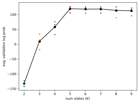
There’s no right answer for how to choose the number of states, but reasonable heuristics include:
picking \(K\) that has the highest average validation log prob
picking \(K\) where the average validation log prob stops increasing by a minimum amount
picking \(K\) with a hypothesis test for increasing mean
Here, we’ll just choose the number of states with the highest average.
best_num_states = all_num_states[jnp.argmax(jnp.stack(avg_val_lls))]
print("best number of states:", best_num_states)
best number of states: 5
Now fit a model to all the training data using the chosen number of states#
# Initialize the parameters using K-Means on the full training set
key = jr.PRNGKey(0)
test_hmm = GaussianHMM(best_num_states, emission_dim, transition_matrix_stickiness=10.)
params, props = test_hmm.initialize(key=key, method="kmeans", emissions=train_emissions)
params, lps = test_hmm.fit_em(params, props, train_emissions, num_iters=100)
Plot the log probabilities over the course of training, along with those of the model with the parameters that generated the data.
# Evaluate the log probability of the training data under the true parameters
true_lp = vmap(partial(hmm.marginal_log_prob, true_params))(train_emissions).sum()
true_lp += hmm.log_prior(true_params)

# Plot log probs vs num_iterations
offset = 0
plt.plot(jnp.arange(len(lps)-offset), lps[offset:], label='EM')
plt.axhline(true_lp, color='k', linestyle=':', label="True")
plt.xlabel('num epochs')
plt.ylabel('log prob')
plt.legend()
<matplotlib.legend.Legend at 0x7fa95c6dabd0>
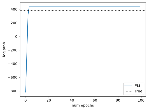
Note
Note that the fitted model can achieve higher log probability than the true model on the training data. Just because the data was generated using these parameters, it doesn’t mean that the true parameters achieve the maximum likelihood for a finite dataset. As the size of the dataset increases, the gap should decrease.
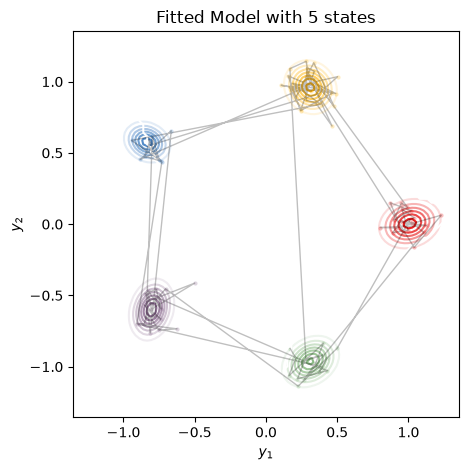
Visualize the fitted model#
We’ll make the same plots as above, but now using the fitted parameters and the chosen number of states.
most_likely_states = test_hmm.most_likely_states(params, train_emissions[0])
plot_gaussian_hmm(test_hmm, params, train_emissions[0], most_likely_states,
                  title=f"Fitted Model with {best_num_states} states", alpha=0.25)
plot_gaussian_hmm_data(test_hmm, params, train_emissions[0], most_likely_states, xlim=(0, 100))
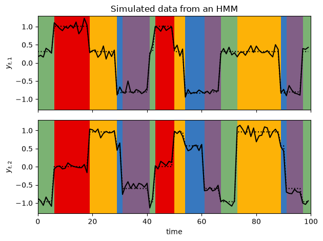
Important
Note that the marginal log probability is invariant to relabeling of the states. Compare these plots to the ones at the top from the true model. You’ll see that the states have been permuted.
Comparing Gaussian HMMs with different constraints on the covariance#
Dynamax implements Gaussian HMMs with different constraints on the covariance matrices:
DiagonalGaussianHMMassumes the covariance matrices are diagonal (i.e. \(\Sigma_k = \mathrm{diag}([\sigma_{k,1}^2, \ldots, \sigma_{k,D}^2])\))SphericalGaussianHMMassumes the covariance matrices are “spherical” (i.e. \(\Sigma_k = \sigma_k^2 I\))SharedCovarianceGaussianHMMassumes the covariance matrices are the same for all states (i.e. \(\Sigma_k = \Sigma\)). Here, \(\Sigma\) can be an arbitrary covariance matrix (not just spherical or diagonal).
In this last section, we will compare these models based on the marginal probability they assign to the test data.
Warning
Usually, you would use cross-validation to choose the number of discrete states for each type of model, and then evaluate them on test data. For simplicity, we will assume that we know the true number of states.
def fit_model(model, key, num_iters=100):
    # Initialize the parameters using K-Means on the full training set
    params, props = model.initialize(key=key, method="kmeans", emissions=train_emissions)
    params, lps = model.fit_em(params, props, train_emissions, num_iters=num_iters, verbose=False)
    test_lp = vmap(partial(model.marginal_log_prob, params))(test_emissions).sum()
    return test_lp

models = [
    GaussianHMM(true_num_states, emission_dim, transition_matrix_stickiness=10.),
    DiagonalGaussianHMM(true_num_states, emission_dim, transition_matrix_stickiness=10.),
    SphericalGaussianHMM(true_num_states, emission_dim, transition_matrix_stickiness=10.),
    SharedCovarianceGaussianHMM(true_num_states, emission_dim, transition_matrix_stickiness=10.),
]

# Fit the models and collect the test log probabilities
key = jr.PRNGKey(0)
test_lps = [fit_model(model, key) for model in models]
# Compare to the log probability under the true model
true_test_lp = vmap(partial(hmm.marginal_log_prob, true_params))(test_emissions).sum()

print("Marginal log probabilities of test data:")
for model, test_lp in zip(models, test_lps):
    print(f"{model.__class__.__name__: >30}: {test_lp: .1f}")
print(f"{'True Model': >30}: {true_test_lp: .1f}")
Marginal log probabilities of test data:
                   GaussianHMM:  106.8
           DiagonalGaussianHMM:  113.5
          SphericalGaussianHMM:  110.8
   SharedCovarianceGaussianHMM:  112.4
                    True Model:  117.5
Here, the DiagonalGaussianHMM has the highest test log likelihood, and it’s almost as high as the log probability under the true parameters. The standard GaussianHMM, which allows for arbitrary covariance matrices is underperforming on test data, likely because it overfits the training data with its extra flexibility.
Here, the true parameters were in fact spherical and shared across all states, so it’s perhaps a bit surprising that the more general diagonal covariance model wins out on test data. Keep in mind, however, that there is some amount of randomness in both the sampled data and the initialization of these models, so the particular ordering might change from one random seed to the next. In actual applications, you should compute means and standard errors by running these analyses with multiple random seeds.
Conclusion#
Dynamax provides a family of Gaussian HMMs for multivariate continuous emissions. This notebook showed how to use cross-validation to choose the number of discrete states, and how to compare model families (e.g. GaussianHMM vs DiagonalGaussianHMM) on test data.
Now that you have seen HMMs with categorical and Gaussian emissions, you can pattern-match to use the other HMMs. See the documentation for a complete list.
The next notebook highlights one more generalization of the standard HMM to autoregressive emissions, where the emissions depend on preceding emissions as well as the current discrete state.