Online learning for an MLP using extended Kalman filtering

We perform sequential (recursive) Bayesian inference for the parameters of a multi layer perceptron (MLP) using the extended Kalman filter. To do this, we treat the parameters of the model as the unknown hidden states. We assume that these are approximately constant over time (we add a small amount of Gaussian drift, for numerical stability.) The graphical model is shown below.

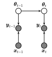
The model has the following form

\[\begin{align*} \theta_t &= \theta_{t-1} + q_t, \; q_t \sim \mathrm{N}(0, 0.01 I) \\ y_t &= h(\theta_t, x_t) + r_t, \; r_t \sim \mathrm{N}(0, \sigma^2) \end{align*}\]

This is a NLG-SSM, where \(h\) is the nonlinear observation model. For details, see sec 17.5.2 of Probabilistic Machine Learning: Advanced Topics.

For a video of the training in action see, https://github.com/probml/probml-data/blob/main/data/ekf_mlp_demo.mp4

Setup

%%capture
try:
    import dynamax
except ModuleNotFoundError:
    print('installing dynamax')
    %pip install -q dynamax[notebooks]
    import dynamax

import jax.numpy as jnp
import flax.linen as nn
import jax.random as jr
import matplotlib.pyplot as plt

from jax import vmap
from jax.flatten_util import ravel_pytree
from typing import Sequence
from functools import partial

from dynamax.nonlinear_gaussian_ssm import ParamsNLGSSM, extended_kalman_filter

Data

Generate noisy observations of a nonlinear function,

\[\begin{align*} y_i &\sim \mathrm{N}(f(x_i), \sigma_y^2) \\ f(x) &= x - 10 \cos(x) \sin(x) + x^3 \end{align*}\]

where the inputs or covariates \(x_i\) are set to,

\[\begin{align*} x_i &\sim \mathrm{N}\left(-3 + 6 \tfrac{i}{n}, \sigma_x^2 \right) \end{align*}\]

Here, we have \(n=200\) observations with noise standard deviations \(\sigma_x = 0.1\) and \(\sigma_y = 3.0\).

The indices of the training pairs \((x_i, y_i)\) are permuted before training so that the network “sees” data points in random order.

def sample_observations(f, x_min, x_max, x_std=0.1, y_std=3.0, num_obs=200, key=0):
    """Generate random training set for MLP given true function and
    distribution parameters.
    Args:
        f (Callable): True function.
        x_min (float): Min x-coordinate to sample from.
        x_max (float): Max x-coordinate to sample from.
        x_std (float, optional): Sampling standard deviation in x-coordinate. Defaults to 0.1.
        y_std (float, optional): Sampling standard deviation in y-coordinate. Defaults to 3.0.
        num_obs (int, optional): Number of training data to generate. Defaults to 200.
        key (int, optional): Random key. Defaults to 0.
    Returns:
        x (num_obs,): x-coordinates of generated data
        y (num_obs,): y-coordinates of generated data
    """
    if isinstance(key, int):
        key = jr.PRNGKey(key)
    keys = jr.split(key, 3)

    # Generate noisy x coordinates
    x_noise = jr.normal(keys[0], (num_obs,)) * x_std
    x = jnp.linspace(x_min, x_max, num_obs) + x_noise

    # Generate noisy y coordinates
    y_noise = jr.normal(keys[1], (num_obs,)) * y_std
    y = f(x) + y_noise

    # Random shuffle (x, y) coordinates
    shuffled_idx = jr.permutation(keys[2], jnp.arange(num_obs))
    x, y = x[shuffled_idx], y[shuffled_idx]
    return x, y

# Generate training set.
# Note that we view the x-coordinates of training data as control inputs
# and the y-coordinates of training data as emissions.
f = lambda x: x - 10 * jnp.cos(x) * jnp.sin(x) + x**3
y_std = 3.0
inputs, emissions = sample_observations(f, x_min=-3, x_max=3, y_std=y_std)

Neural network

We aim to approximate the true data generating function, \(f(x)\), with a parametric approximation, \(h(\theta, x)\), where \(\theta\) are the parameters and \(x\) are the inputs. We use a simple feedforward neural network — a.k.a. multi-layer perceptron (MLP) — with sigmoidal noinlinearities. Here, \(\theta\) corresponds to the flattened vector of all the weights from all the layers of the model.

class MLP(nn.Module):
    features: Sequence[int]

    @nn.compact
    def __call__(self, x):
        for feat in self.features[:-1]:
            x = nn.sigmoid(nn.Dense(feat)(x))
        x = nn.Dense(self.features[-1])(x)
        return x

def get_mlp_flattened_params(model_dims, key=0):
    """Generate MLP model, initialize it using dummy input, and
    return the model, its flattened initial parameters, function
    to unflatten parameters, and apply function for the model.
    Args:
        model_dims (List): List of [input_dim, hidden_dim, ..., output_dim]
        key (PRNGKey): Random key. Defaults to 0.
    Returns:
        model: MLP model with given feature dimensions.
        flat_params: Flattened parameters initialized using dummy input.
        unflatten_fn: Function to unflatten parameters.
        apply_fn: fn(flat_params, x) that returns the result of applying the model.
    """
    if isinstance(key, int):
        key = jr.PRNGKey(key)

    # Define MLP model
    input_dim, features = model_dims[0], model_dims[1:]
    model = MLP(features)
    dummy_input = jnp.ones((input_dim,))

    # Initialize parameters using dummy input
    params = model.init(key, dummy_input)
    flat_params, unflatten_fn = ravel_pytree(params)

    # Define apply function
    def apply(flat_params, x, model, unflatten_fn):
        return model.apply(unflatten_fn(flat_params), jnp.atleast_1d(x))

    apply_fn = partial(apply, model=model, unflatten_fn=unflatten_fn)

    return model, flat_params, unflatten_fn, apply_fn

input_dim, hidden_dim, output_dim = 1, 6, 1
model_dims = [input_dim, hidden_dim, output_dim]
_, flat_params, _, apply_fn = get_mlp_flattened_params(model_dims)

Online inference

Here we demonstrate how to estimate the model parameters in online fashion using the Extended Kalman Filter (EKF). As described above, the idea is to think of the latent state as the parameter estimate at time \(t\), after seeing \(t\) data points. Each new data point provides an update of the parameter estimate, and the parameters are allowed to drift very slightly from one data point to the next. (In this simulated example, the true parameters are constant throughout, so the EKF is actually a bit more flexible than necessary.)

# Note that the dynamics function is the identity function
# and the emission function is the model apply function
state_dim, emission_dim = flat_params.size, output_dim
ekf_params = ParamsNLGSSM(
    initial_mean=flat_params,
    initial_covariance=jnp.eye(state_dim) * 100,
    dynamics_function=lambda x, u: x,
    dynamics_covariance=jnp.eye(state_dim) * 1e-4,
    emission_function=apply_fn,
    emission_covariance=jnp.eye(emission_dim) * y_std**2,
)

# Run EKF on training set to train MLP
ekf_post = extended_kalman_filter(ekf_params, emissions, inputs=inputs)
w_means, w_covs = ekf_post.filtered_means, ekf_post.filtered_covariances

Plot results

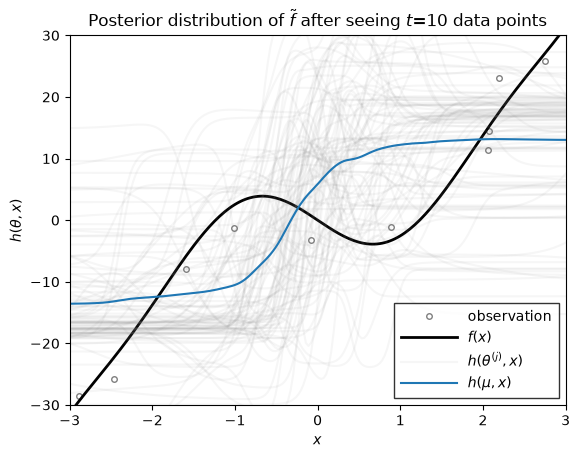
Let \(h(\theta, x)\) denote the function approximation produced by an MLP with parameters \(\theta\). If we the parameters are random, \(\theta \sim \mathrm{N}(\mu, \Sigma)\), then the resulting function \(h\) is random as well. We can visualize the distribution over functions by drawing samples of \(\theta\) and plotting the resulting function for each parameter sample.

The helper function below plots \(h(\mu, x)\) in blue, where \(\mu\) is the mean of the parameter distribution. It also plots the function for various parameter samples \(h(\theta^{(j)}, x)\) where \(\theta^{(j)} \sim \mathrm{N}(\mu, \Sigma)\). These samples give a sense of the uncertainty of \(h\) under the distribution of parameters.

def plot_mlp_prediction(f, h, obs, x_grid, w_mean, w_cov, ax, num_samples=100, x_lim=(-3, 3), y_lim=(-30, 30), key=0):
    if isinstance(key, int):
        key = jr.PRNGKey(key)

    # Plot observations (training set)
    ax.plot(obs[0], obs[1], "ok", fillstyle="none", ms=4, alpha=0.5, label="observation")

    # Plot the true function on a grid of points
    ax.plot(x_grid, vmap(f)(x_grid), linewidth=2, label=r"$f(x)$", color='k')

    # Indicate uncertainty through sampling
    w_samples = jr.multivariate_normal(key, w_mean, w_cov, (num_samples,))
    y_samples = vmap(vmap(h, in_axes=(None, 0)), in_axes=(0, None))(w_samples, x_grid)
    for j, y_sample in enumerate(y_samples):
        ax.plot(x_grid, y_sample, color="gray", alpha=0.07, 
                label=r"$h(\theta^{(j)}, x)$" if j==0 else None)

    # Plot prediction on grid using filtered mean of MLP params
    # y_mean = vmap(h, in_axes=(None, 0))(w_mean, x_grid)
    y_mean = y_samples.mean(axis=0)
    ax.plot(x_grid, y_mean, linewidth=1.5, label=r"$h(\mu, x)$")

    ax.set_xlim(x_lim)
    ax.set_ylim(y_lim)
    ax.set_xlabel(r"$x$")
    ax.set_ylabel(r"$h(\theta, x)$")
    ax.legend(loc=4, borderpad=0.5, handlelength=4, fancybox=False, edgecolor="k")

Plot the estimated function after seeing different numbers of data points

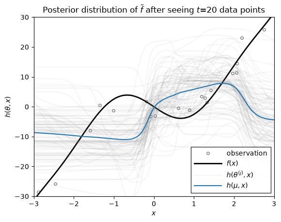
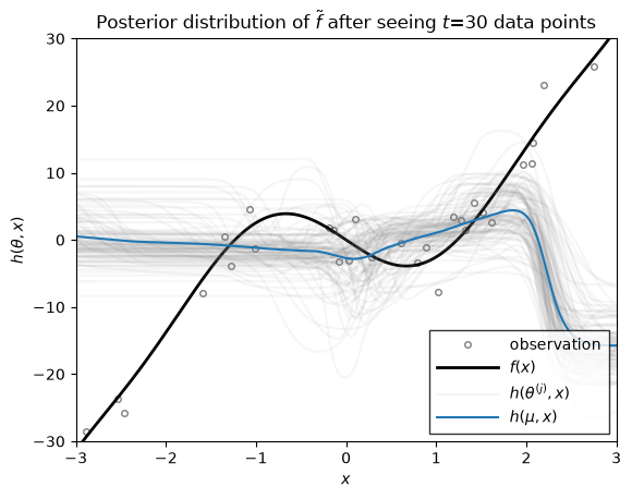
Now we we use the function above to plot the distribution over functions, \(h\), under the filtering distribution of the parameters \(\theta_t \sim \mathrm{N}(\mu_{t|t}, \Sigma_{t|t})\), where the mean and covariance are from the extended Kalman filter above. These distributions capture the uncertainty in \(h\) after seeing \(t\) data points.

all_figures = {}
inputs_grid = jnp.linspace(inputs.min(), inputs.max(), len(inputs))
intermediate_steps = [10, 20, 30, 200]
for step in intermediate_steps:
    print('ntraining =', step)
    fig, ax = plt.subplots()
    plot_mlp_prediction(f, 
        apply_fn, (inputs[:step], emissions[:step]), inputs_grid, w_means[step - 1], w_covs[step - 1], ax, key=step
    )
    ax.set_title(rf"Posterior distribution of $\tilde{{f}}$ after seeing $t$={step} data points")
    all_figures[f"ekf_mlp_step_{step}"] = fig

ntraining = 10

ntraining = 20
ntraining = 30
ntraining = 200

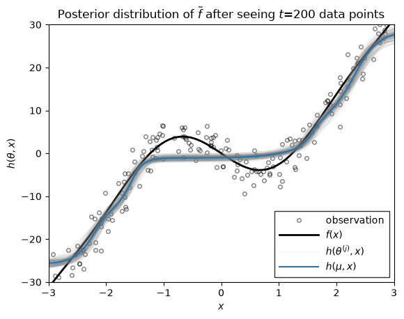
Conclusion

As you can see, as the number of data points grows, the posterior distribution over functions concentrates. At early stages, the EKF appears to be overly confident in its predictions, sometimes in the face of data. By the time 200 data points have been observed, however, the estimate does a good job of approximating the true data-generating function!