What are State Space Models?
What are State Space Models?
A state space model or SSM is a partially observed Markov model, in which the hidden state, \(\hidden_t\), evolves over time according to a Markov process, possibly conditional on external inputs or controls \(\input_t\), and each hidden state generates some observations \(\obs_t\) at each time step. (In this book, we mostly focus on discrete time systems, although we consider the continuous-time case in XXX.) We get to see the observations, but not the hidden state. Our main goal is to infer the hidden state given the observations. However, we can also use the model to predict future observations, by first predicting future hidden states, and then predicting what observations they might generate. By using a hidden state \(\hidden_t\) to represent the past observations, \(\obs_{1:t-1}\), the model can have ``infinite’’ memory, unlike a standard Markov model.
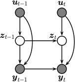
Fig. 1 Illustration of an SSM as a graphical model.
Formally we can define an SSM as the following joint distribution:
where \(p(\hidden_t|\hidden_{t-1},\inputs_t)\) is the transition model, \(p(\obs_t|\hidden_t, \inputs_t, \obs_{t-1})\) is the observation model, and \(\inputs_{t}\) is an optional input or action. See Fig. 1 for an illustration of the corresponding graphical model.
We often consider a simpler setting in which the observations are conditionally independent of each other (rather than having Markovian dependencies) given the hidden state. In this case the joint simplifies to
Sometimes there are no external inputs, so the model further simplifies to the following unconditional generative model:
See Fig. 2 for an illustration of the corresponding graphical model.
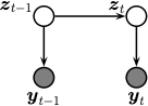
Fig. 2 Illustration of a simplified SSM.
SSMs are widely used in many areas of science, engineering, finance, economics, etc. The main applications are state estimation (i.e., inferring the underlying hidden state of the system given the observation), forecasting (i.e., predicting future states and observations), and control (i.e., inferring the sequence of inputs that will give rise to a desired target state). We will discuss these applications in later chapters.