Parameter estimation (learning)
### Import standard libraries

import abc
from dataclasses import dataclass
import functools
from functools import partial
import itertools
import matplotlib.pyplot as plt
import numpy as np
from typing import Any, Callable, NamedTuple, Optional, Union, Tuple

import jax
import jax.numpy as jnp
from jax import lax, vmap, jit, grad
#from jax.scipy.special import logit
#from jax.nn import softmax
import jax.random as jr


import distrax
import optax

import jsl
import ssm_jax
Parameter estimation (learning)
So far, we have assumed that the parameters \(\params\) of the SSM are known. For example, in the case of an HMM with categorical observations we have \(\params = (\hmmInit, \hmmTrans, \hmmObs)\), and in the case of an LDS, we have \(\params = (\ldsTrans, \ldsObs, \ldsTransIn, \ldsObsIn, \transCov, \obsCov, \initMean, \initCov)\). If we adopt a Bayesian perspective, we can view these parameters as random variables that are shared across all time steps, and across all sequences. This is shown in Fig. 6, where we adopt \(\keyword{plate notation}\) to represent repetitive structure.
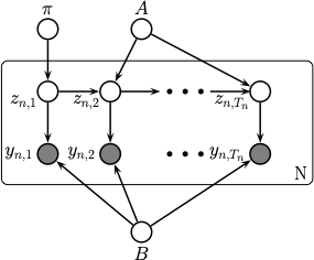
Fig. 6 Illustration of an HMM using plate notation, where we show the parameter nodes which are shared across all the sequences.
Suppose we observe \(N\) sequences \(\data = \{\obs_{n,1:T_n}: n=1:N\}\). Then the goal of \(\keyword{parameter estimation}\), also called \(\keyword{model learning}\) or \(\keyword{model fitting}\), is to approximate the posterior
where \(p(\obs_{n,1:T_n} | \params)\) is the marginal likelihood of sequence \(n\):
Since computing the full posterior is computationally difficult, we often settle for computing a point estimate such as the MAP (maximum a posterior) estimate
If we ignore the prior term, we get the maximum likelihood estimate or MLE:
In practice, the MAP estimate often works better than the MLE, since the prior can regularize the estimate to ensure the model is numerically stable and does not overfit the training set.
We will discuss a variety of algorithms for parameter estimation in later chapters.