Linear Gaussian SSMs
Contents
### Import standard libraries

import abc
from dataclasses import dataclass
import functools
from functools import partial
import itertools
import matplotlib.pyplot as plt
import numpy as np
from typing import Any, Callable, NamedTuple, Optional, Union, Tuple

import jax
import jax.numpy as jnp
from jax import lax, vmap, jit, grad
#from jax.scipy.special import logit
#from jax.nn import softmax
import jax.random as jr


import distrax
import optax

import jsl
import ssm_jax

import inspect
import inspect as py_inspect
import rich
from rich import inspect as r_inspect
from rich import print as r_print

def print_source(fname):
    r_print(py_inspect.getsource(fname))
Linear Gaussian SSMs
Consider the state space model in (1) where we assume the observations are conditionally iid given the hidden states and inputs (i.e. there are no auto-regressive dependencies between the observables). We can rewrite this model as a stochastic \(\keyword{nonlinear dynamical system}\) or \(\keyword{NLDS}\) by defining the distribution of the next hidden state \(\hidden_t \in \real^{\nhidden}\) as a deterministic function of the past state \(\hidden_{t-1}\), the input \(\inputs_t \in \real^{\ninputs}\), and some random \(\keyword{process noise}\) \(\transNoise_t \in \real^{\nhidden}\)
where \(\transNoise_t\) is drawn from the distribution such that the induced distribution on \(\hidden_t\) matches \(p(\hidden_t|\hidden_{t-1}, \inputs_t)\). Similarly we can rewrite the observation distribution as a deterministic function of the hidden state plus \(\keyword{observation noise}\) \(\obsNoise_t \in \real^{\nobs}\):
If we assume additive Gaussian noise, the model becomes
where \(\transNoise_t \sim \gauss(\vzero,\transCov_t)\) and \(\obsNoise_t \sim \gauss(\vzero,\obsCov_t)\). We will call these \(\keyword{Gaussian SSMs}\).
If we additionally assume the transition function \(\dynamicsFn\) and the observation function \(\measurementFn\) are both linear, then we can rewrite the model as follows:
This is called a \(\keyword{linear-Gaussian state space model}\) or \(\keyword{LG-SSM}\); it is also called a \(\keyword{linear dynamical system}\) or \(\keyword{LDS}\). We usually assume the parameters are independent of time, in which case the model is said to be time-invariant or homogeneous.
Example: tracking a 2d point
Consider an object moving in \(\real^2\). Let the state be the position and velocity of the object, \(\hidden_t =\begin{pmatrix} u_t & \dot{u}_t & v_t & \dot{v}_t \end{pmatrix}\). (We use \(u\) and \(v\) for the two coordinates, to avoid confusion with the state and observation variables.) If we use Euler discretization, the dynamics become
where \(\transNoise_t \sim \gauss(\vzero,\transCov)\) is the process noise. We assume that the process noise is a white noise process added to the velocity components of the state, but not to the location, so \(\transCov = \diag(0, q, 0, q)\). This is known as a random accelerations model. (See [Sar13] p60 for a more accurate way to convert the continuous time process to discrete time.)
Now suppose that at each discrete time point we observe the location, corrupted by Gaussian noise. Thus the observation model becomes
where \(\obsNoise_t \sim \gauss(\vzero,\obsCov)\) is the observation noise. We see that the observation matrix \(\ldsObs\) simply ``extracts’’ the relevant parts of the state vector.
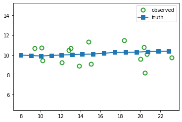
Suppose we sample a trajectory and corresponding set of noisy observations from this model, \((\hidden_{1:T}, \obs_{1:T}) \sim p(\hidden,\obs|\params)\). (We use diagonal observation noise, \(\obsCov = \diag(\sigma_1^2, \sigma_2^2)\).) The results are shown below.
key = jax.random.PRNGKey(314)
timesteps = 15
delta = 1.0
A = jnp.array([
    [1, 0, delta, 0],
    [0, 1, 0, delta],
    [0, 0, 1, 0],
    [0, 0, 0, 1]
])

C = jnp.array([
    [1, 0, 0, 0],
    [0, 1, 0, 0]
])

state_size, _ = A.shape
observation_size, _ = C.shape

Q = jnp.eye(state_size) * 0.001
R = jnp.eye(observation_size) * 1.0
# Prior parameter distribution
mu0 = jnp.array([8, 10, 1, 0]).astype(float)
Sigma0 = jnp.eye(state_size) * 1.0

from jsl.lds.kalman_filter import LDS, smooth, filter

lds = LDS(A, C, Q, R, mu0, Sigma0)
print(lds)
WARNING:absl:No GPU/TPU found, falling back to CPU. (Set TF_CPP_MIN_LOG_LEVEL=0 and rerun for more info.)
LDS(A=DeviceArray([[1., 0., 1., 0.],
             [0., 1., 0., 1.],
             [0., 0., 1., 0.],
             [0., 0., 0., 1.]], dtype=float32), C=DeviceArray([[1, 0, 0, 0],
             [0, 1, 0, 0]], dtype=int32), Q=DeviceArray([[0.001, 0.   , 0.   , 0.   ],
             [0.   , 0.001, 0.   , 0.   ],
             [0.   , 0.   , 0.001, 0.   ],
             [0.   , 0.   , 0.   , 0.001]], dtype=float32), R=DeviceArray([[1., 0.],
             [0., 1.]], dtype=float32), mu=DeviceArray([ 8., 10.,  1.,  0.], dtype=float32), Sigma=DeviceArray([[1., 0., 0., 0.],
             [0., 1., 0., 0.],
             [0., 0., 1., 0.],
             [0., 0., 0., 1.]], dtype=float32), state_offset=None, obs_offset=None, nstates=4, nobs=2)
from jsl.demos.plot_utils import plot_ellipse

def plot_tracking_values(observed, filtered, cov_hist, signal_label, ax):
    timesteps, _ = observed.shape
    ax.plot(observed[:, 0], observed[:, 1], marker="o", linewidth=0,
            markerfacecolor="none", markeredgewidth=2, markersize=8, label="observed", c="tab:green")
    ax.plot(*filtered[:, :2].T, label=signal_label, c="tab:red", marker="x", linewidth=2)
    for t in range(0, timesteps, 1):
        covn = cov_hist[t][:2, :2]
        plot_ellipse(covn, filtered[t, :2], ax, n_std=2.0, plot_center=False)
    ax.axis("equal")
    ax.legend()
z_hist, x_hist = lds.sample(key, timesteps)

fig_truth, axs = plt.subplots()
axs.plot(x_hist[:, 0], x_hist[:, 1],
        marker="o", linewidth=0, markerfacecolor="none",
        markeredgewidth=2, markersize=8,
        label="observed", c="tab:green")

axs.plot(z_hist[:, 0], z_hist[:, 1],
        linewidth=2, label="truth",
        marker="s", markersize=8)
axs.legend()
axs.axis("equal")
(7.24486608505249, 23.857812213897706, 8.042076778411865, 11.636079120635987)
The main task is to infer the hidden states given the noisy observations, i.e., \(p(\hidden_t|\obs_{1:t},\params)\) or \(p(\hidden_t|\obs_{1:T}, \params)\) in the offline case. We discuss the topic of inference in States estimation (inference). We will usually represent this belief state by a Gaussian distribution, \(p(\hidden_t|\obs_{1:s},\params) = \gauss(\hidden_t| \mean_{t|s}, \covMat_{t|s})\), where usually \(s=t\) or \(s=T\). Sometimes we use information form, \(p(\hidden_t|\obs_{1:s},\params) = \gaussInfo(\hidden_t|\precMean_{t|s}, \precMat_{t|s})\).