.ipynb .pdf

repository open issue

Binder Colab

Contents

# meta-data does not work yet in VScode
# https://github.com/microsoft/vscode-jupyter/issues/1121

{
    "tags": [
        "hide-cell"
    ]
}


### Install necessary libraries

try:
    import jax
except:
    # For cuda version, see https://github.com/google/jax#installation
    %pip install --upgrade "jax[cpu]" 
    import jax

try:
    import distrax
except:
    %pip install --upgrade  distrax
    import distrax

try:
    import jsl
except:
    %pip install git+https://github.com/probml/jsl
    import jsl

try:
    import rich
except:
    %pip install rich
    import rich

{
    "tags": [
        "hide-cell"
    ]
}


### Import standard libraries

import abc
from dataclasses import dataclass
import functools
import itertools

from typing import Any, Callable, NamedTuple, Optional, Union, Tuple

import matplotlib.pyplot as plt
import numpy as np


import jax
import jax.numpy as jnp
from jax import lax, vmap, jit, grad
from jax.scipy.special import logit
from jax.nn import softmax
from functools import partial
from jax.random import PRNGKey, split

import inspect
import inspect as py_inspect
import rich
from rich import inspect as r_inspect
from rich import print as r_print

def print_source(fname):
    r_print(py_inspect.getsource(fname))

Nonlinear Gaussian SSMs

In this section, we consider SSMs in which the dynamics and/or observation models are nonlinear, but the process noise and observation noise are Gaussian. That is,

(10)\[\begin{align} \hidden_t &= \dynamicsFn(\hidden_{t-1}, \inputs_t) + \transNoise_t \\ \obs_t &= \obsFn(\hidden_{t}, \inputs_t) + \obsNoise_t \end{align}\]

where \(\transNoise_t \sim \gauss(\vzero,\transCov)\) and \(\obsNoise_t \sim \gauss(\vzero,\obsCov)\). This is a very widely used model class. We give some examples below.

Example: tracking a 1d pendulum

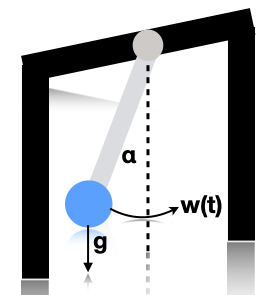
Fig. 4 Illustration of a pendulum swinging. \(g\) is the force of gravity, \(w(t)\) is a random external force, and \(\alpha\) is the angle wrt the vertical. Based on [Sar13] fig 3.10.

Consider a simple pendulum of unit mass and length swinging from a fixed attachment, as in Fig. 4. Such an object is in principle entirely deterministic in its behavior. However, in the real world, there are often unknown forces at work (e.g., air turbulence, friction). We will model these by a continuous time random Gaussian noise process \(w(t)\). This gives rise to the following differential equation:

(11)\[\begin{align} \frac{d^2 \alpha}{d t^2} = -g \sin(\alpha) + w(t) \end{align}\]

We can write this as a nonlinear SSM by defining the state to be \(\hidden_1(t) = \alpha(t)\) and \(\hidden_2(t) = d\alpha(t)/dt\). Thus

(12)\[\begin{align} \frac{d \hidden}{dt} = \begin{pmatrix} \hiddenScalar_2 \\ -g \sin(\hiddenScalar_1) \end{pmatrix} + \begin{pmatrix} 0 \\ 1 \end{pmatrix} w(t) \end{align}\]

If we discretize this step size \(\Delta\), we get the following formulation [Sar13] p74:

(13)\[\begin{align} \underbrace{ \begin{pmatrix} \hiddenScalar_{1,t} \\ \hiddenScalar_{2,t} \end{pmatrix} }_{\hidden_t} = \underbrace{ \begin{pmatrix} \hiddenScalar_{1,t-1} + \hiddenScalar_{2,t-1} \Delta \\ \hiddenScalar_{2,t-1} -g \sin(\hiddenScalar_{1,t-1}) \Delta \end{pmatrix} }_{\dynamicsFn(\hidden_{t-1})} +\transNoise_{t-1} \end{align}\]

where \(\transNoise_{t-1} \sim \gauss(\vzero,\transCov)\) with

(14)\[\begin{align} \transCov = q^c \begin{pmatrix} \frac{\Delta^3}{3} & \frac{\Delta^2}{2} \\ \frac{\Delta^2}{2} & \Delta \end{pmatrix} \end{align}\]

where \(q^c\) is the spectral density (continuous time variance) of the continuous-time noise process.

If we observe the angular position, we get the linear observation model \(\obsFn(\hidden_t) = \alpha_t = \hiddenScalar_{1,t}\). If we only observe the horizontal position, we get the nonlinear observation model \(\obsFn(\hidden_t) = \sin(\alpha_t) = \sin(\hiddenScalar_{1,t})\).

previous

Linear Gaussian SSMs

next

States estimation (inference)